ВЉЮФ
етЦЊNatureзгПЏЮФеТЕФЕААззщбЇЪ§ОнPCAЗжЮіОЙЛЈЗбСЫЮвСНЬьЪБМфРДжиЯж|ИНШЋЙ§ГЬДњТы
||
2020Фъ4дТ14ШеЃЌSangerбаОПЭХЖггкnature communicationдкЯпЗЂБэСЫЬтЮЊSingle-cell transcriptomics identifies an effectorness gradient shaping the response of CD4+ T cells to cytokinesЕФбаОПФкШнЃЌзїепЪЙгУЕААзжЪзщбЇЁЂbulk RNA-seqКЭЕЅЯИАћзЊТМзщВтађЖдШЫЬх40,000ИівдЩЯЕФnaïve and memory CD4+ T cellsНјааЗжЮіЃЌЗЂЯжЯИАћРраЭжЎМфЕФЯИАћвђзгЗДгІВювьКмДѓЁЃmemory TЯИАћВЛФмЗжЛЏЮЊTh2БэаЭЃЌЕЋПЩвдЯьгІiTregМЋЛЏЛёЕУРрЫЦTh17ЕФБэаЭЁЃЕЅЯИАћЗжЮіБэУїЃЌTЯИАћЙЙГЩСЫвЛИізЊТМСЌајЬхЃЈtranscriptional continuumЃЉЃЌДггзжЩЕНжаЪрКЭаЇгІМЧвфTЯИАћЃЌаЮГЩСЫвЛжжаЇгІЬнЖШЃЌВЂАщЫцзХЧїЛЏвђзгКЭЯИАћвђзгБэДяЕФдіМгЁЃзюКѓЃЌзїепБэУїЃЌTЯИАћЛюЛЏКЭЯИАћвђзгЗДгІЪмаЇгІЬнЖШЕФгАЯьЁЃ
ИУЮФЯзЭЈЙ§ЕААзжЪзщбЇЃЈ(вКЯрЩЋЦз-ДЎСЊжЪЦзЗЈЃЌLC-MS/MSЃЉНјааСЫЬНЫїадЗжЮіЃЌбљЦЗЖдгІгкДгНЁПЕИіЬхЕФЭтжмбЊжаЗжРыЕФгзжЩКЭМЧвфTЯИАћЃЌВЂгУЖржжЯИАћвђзгДЬМЄ5ЬьЃЌУПИіЬѕМўЦНОљ3ИіЩњЮябЇжиИДЁЃ
етДЮИДЯжFig1cPCAЭМКЭFig2aPCAЭМЕФСэвЛВПЗжЃЌетДЮзїепЪЧЭЈЙ§ЕААззщбЇЪ§ОнНјааPCAЕФеЙЯжЃК
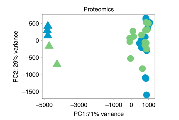
вдЩЯЪЧFig1cдЭМЃЌЭМзЂЮЊЁАPCA plots from the whole transcriptome of TN and TM cells. Different colors correspond to cell types and different shades to stimulation time points. PCA plots were derived using 21 naive and 19 memory T cell samples for proteomicsЁБ
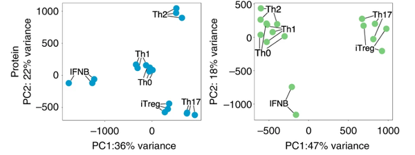
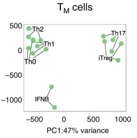
вдЩЯЮЊFig 2aдЭМЃЌЭМзЂЮЊЁАPCA plot from the full transcriptome of TN and TM cells following five days of cytokine stimulations. Only stimulated cells were included in this analysis. PCA plots were derived using 18 naive and 17 memory T cells samples ЁБ
ЮвУЧашвЊИДЯжИУЭМжЎЧАЃЌЯШашвЊЯТдиЪ§ОнЃЌПЩвдЕуЛїhttps://www.opentargets.org/projects/effectornessЖдproteomicsЕФabundancesЪ§ОнКЭmetadataЪ§ОнНјааЯТдиЃЌШЛКѓНјаавдЯТВНжшЃК
library(SummarizedExperiment)
library(annotables)
library(rafalib)
library(ggplot2)
library(ggrepel)
library(limma)
МгдиЪ§Он
МгдиБъзМЛЏКѓЕФЗсЖШЃК
MassSpec_data <- read.table("NCOMMS-19-7936188_MassSpec_scaled_abundances.txt", header = T, stringsAsFactors = F)
View(MassSpec_data)
#ДгвдЩЯПЩвдПДГіЃЌУПСаГ§СЫДњБэУПИібљБОЭтЃЌЧАШ§СаЗжБ№ЮЊProtein_idЃЌGene_idКЭGene_nameЃЌУПааДњБэвЛИіЕААзНЈСЂSummarizedExperiment object
ДДНЈДјгаЕААзжЪзЂЪЭЕФdataframe
protein_annotations <- data.frame(MassSpec_data[,c("Protein_id","Gene_id","Gene_name")], row.names = MassSpec_data$Gene_name)
rownames(MassSpec_data) <- MassSpec_data$Gene_name#ЙЙГЩвЛИігЩ"Protein_id","Gene_id","Gene_name"ЕФЪ§ОнПђ
MassSpec_data <- MassSpec_data[,-c(1:3)]ДДНЈДјгаsampleзЂЪЭЕФdataframe
sample_ids <- colnames(MassSpec_data)
sample_annotations <- data.frame(row.names = sample_ids,
donor_id = sapply(sample_ids, function(x){strsplit(x, split = "_")[[1]][1]}),
cell_type = paste("CD4",
sapply(sample_ids, function(x){strsplit(x, split = "_")[[1]][3]}),
sep="_"),
cytokine_condition = sapply(sample_ids, function(x){strsplit(x, split = "_")[[1]][4]}),
stringsAsFactors = T)
sample_annotations$activation_status <- ifelse(sample_annotations$cytokine_condition == "resting", "Resting", "Activated")
View(sample_annotations)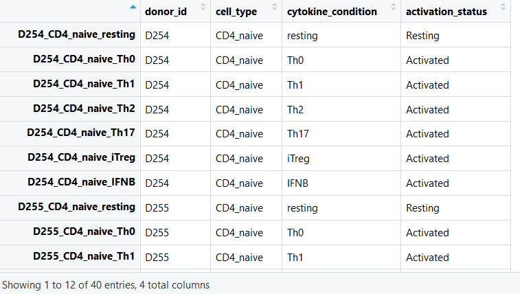
ДДНЈrelevant metadataЕФБфСП
meta <- list(
Study="Mapping cytokine induced gene expression changes in human CD4+ T cells",
Experiment="Quantitative proteomics (LC-MS/MS) panel of cytokine induced T cell polarisations",
Laboratory="Trynka Group, Wellcome Sanger Institute",
Experimenter=c("Eddie Cano-Gamez",
"Blagoje Soskic",
"Deborah Plowman"),
Description="To study cytokine-induced cell polarisation, we isolated human naive and memory CD4+ T cells in triplicate from peripheral blood of healthy individuals. Next, we polarised the cells with different cytokine combinations linked to autoimmunity and performed LC-MS/MS.",
Methdology="LC-MS/MS with isobaric labelling",
Characteristics="Data type: Normalised, scaled protein abundances",
Date="September, 2019",
URL="https://doi.org/10.1101/753731"
)НЈСЂSummarizedExperiment object
proteomics_data <- SummarizedExperiment(assays=list(counts=as.matrix(MassSpec_data)),
colData=sample_annotations,
rowData=protein_annotations,
metadata=meta)
saveRDS(proteomics_data, file="proteinAbundances_summarizedExperiment.rds")
Ъ§ОнПЩЪгЛЏ
НЋNAжЕЩшжУЮЊСузЂвтЃКДЫВйзїНіГігкПЩЪгЛЏФПЕФЁЃжДааЭГМЦВтЪдЪБЃЌNAВЛЛсЩшжУЮЊСуЁЃ
assay(proteomics_data)[is.na(assay(proteomics_data))] <- 0
ЖЈвхКЏЪ§ЃК
ЬсШЁЕААзжЪБэДяжЕ;
НјаажїГЩЗжЗжЮі;
ЗЕЛивЛИіОиеѓЃЌЦфжаАќКЌУПИібљЦЗКЭбљЦЗзЂЪЭЕФPCзјБъ;
ЗЕЛиУПИіжївЊГЩЗжНтЪЭЕФЗНВюАйЗжБШЁЃ
getPCs <- function(exp){
pcs <- prcomp(t(assay(exp)))
pVar <- pcs$sdev^2/sum(pcs$sdev^2)
pca.mat <- data.frame(pcs$x)
pca.mat$donor_id <- colData(exp)$donor_id
pca.mat$cell_type <- colData(exp)$cell_type
pca.mat$cytokine_condition <- colData(exp)$cytokine_condition
pca.mat$activation_status <- colData(exp)$activation_status
res <- list(pcs = pca.mat, pVar=pVar)
return(res)
}ЖдЫљгабљБОжДааPCA
pcs <- getPCs(proteomics_data)ggplot(data=pcs$pcs, aes(x=PC1, y=PC2, color=cell_type, shape=activation_status)) +
geom_point(size = 8) +
xlab(paste0("PC1:", round(pcs$pVar[1]*100), "% variance")) +
ylab(paste0("PC2: ", round(pcs$pVar[2]*100), "% variance")) +
scale_colour_manual(values = c("#5AB4AC","#AF8DC3")) +
scale_alpha_discrete(range = c(0.5,1)) +
coord_fixed() + theme_bw() +
theme(panel.grid = element_blank())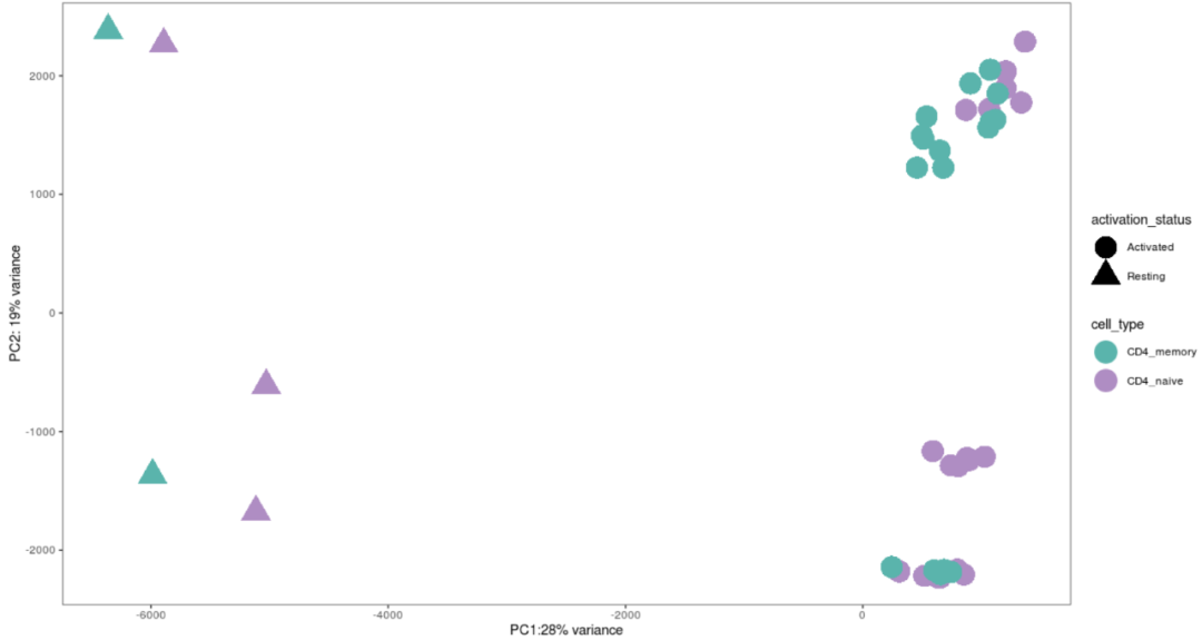
ШЅЕєИіЬхМфБфвьадЃК
proteomics_data_regressed <- proteomics_data
assay(proteomics_data_regressed) <- removeBatchEffect(assay(proteomics_data_regressed),
batch = factor(as.vector(colData(proteomics_data_regressed)$donor_id))
)
жиаТМЦЫуPCAЃК
pcs <- getPCs(proteomics_data_regressed)ggplot(data=pcs$pcs, aes(x=PC1, y=PC2, color=cell_type, shape=activation_status)) +
geom_point(size = 8) +
xlab(paste0("PC1:", round(pcs$pVar[1]*100), "% variance")) +
ylab(paste0("PC2: ", round(pcs$pVar[2]*100), "% variance")) +
scale_colour_manual(values = c("#5AB4AC","#AF8DC3")) +
scale_alpha_discrete(range = c(0.5,1)) +
coord_fixed() + theme_bw() +
theme(panel.grid = element_blank())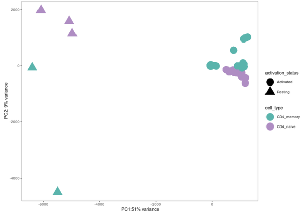
дЭМ
ЯИАћРраЭЬивьадЗжЮі
НЋnaiveКЭmemory TЯИАћбљБОЗжЮЊНіАќКЌЪмДЬМЄЯИАћЕФСНИіВЛЭЌЪ§ОнМЏЁЃ
proteomics_data_naive <- proteomics_data[,(proteomics_data$cell_type=="CD4_naive") & (proteomics_data$activation_status=="Activated")]
proteomics_data_memory <- proteomics_data[,(proteomics_data$cell_type=="CD4_memory") & (proteomics_data$activation_status=="Activated")]
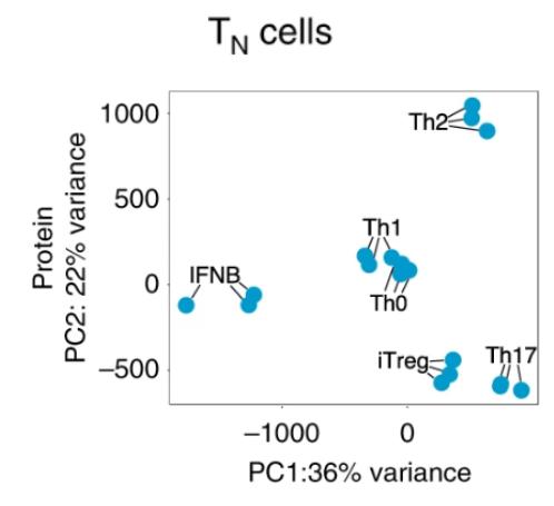
Naive T cells
Жд 5 days-stimulated naive T cellsНјааPCA:
pcs_naive <- getPCs(proteomics_data_naive)
ggplot(data=pcs_naive$pcs, aes(x=PC1, y=PC2)) + geom_point(aes(color=donor_id), size=8) +
xlab(paste0("PC1:", round(pcs_naive$pVar[1]*100), "% variance")) +
ylab(paste0("PC2: ", round(pcs_naive$pVar[2]*100), "% variance")) +
coord_fixed() + theme_bw() +
theme(plot.title=element_text(size=20, hjust=0.5), axis.title=element_text(size=14), panel.grid = element_blank(), axis.text=element_text(size=12),legend.text=element_text(size=12), legend.title=element_text(size=12), legend.key.size = unit(1.5,"lines"))
ШЅЕєИіЬхМфБфвьадЃК
assay(proteomics_data_naive) <- removeBatchEffect(assay(proteomics_data_naive),
batch = factor(as.vector(colData(proteomics_data_naive)$donor_id))
)
pcs_naive <- getPCs(proteomics_data_naive)
ggplot(data=pcs_naive$pcs, aes(x=PC1, y=PC2, color=cytokine_condition)) +
geom_point(size = 8) + geom_label_repel(aes(label=cytokine_condition, color=cytokine_condition)) +
xlab(paste0("PC1: ", round(pcs_naive$pVar[1]*100), "% variance")) +
ylab(paste0("PC2: ", round(pcs_naive$pVar[2]*100), "% variance")) +
scale_colour_brewer(palette = "Dark2") +
scale_fill_brewer(palette = "Dark2") +
coord_fixed() + theme_bw() +
theme(panel.grid = element_blank(), legend.position = "none")
ЩОГ§гЩPCAБъЪЖЕФвьГЃбљБО:
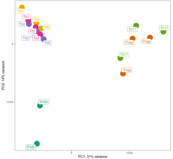
proteomics_data_naive <- proteomics_data_naive[, colnames(proteomics_data_naive) != "D257_CD4_naive_Th1"]pcs_naive <- getPCs(proteomics_data_naive)ggplot(data=pcs_naive$pcs, aes(x=PC1, y=PC2, color=cytokine_condition)) +
geom_point(size = 8) + geom_label_repel(aes(label=cytokine_condition, color=cytokine_condition)) +
xlab(paste0("PC1: ", round(pcs_naive$pVar[1]*100), "% variance")) +
ylab(paste0("PC2: ", round(pcs_naive$pVar[2]*100), "% variance")) +
scale_colour_brewer(palette = "Dark2") +
scale_fill_brewer(palette = "Dark2") +
coord_fixed() + theme_bw() +
theme(panel.grid = element_blank(), legend.position = "none")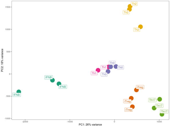
дЭМ
Memory T cells
againЁЃЁЃЁЃ
Performing PCA on 5 days-stimulated memory T cells only.
```{r compute_pca_naive, message=FALSE, warning=FALSE}
pcs_memory <- getPCs(proteomics_data_memory)ggplot(data=pcs_memory$pcs, aes(x=PC1, y=PC2)) + geom_point(aes(color=donor_id), size=8) +
xlab(paste0("PC1:", round(pcs_memory$pVar[1]*100), "% variance")) +
ylab(paste0("PC2: ", round(pcs_memory$pVar[2]*100), "% variance")) +
coord_fixed() + theme_bw() +
theme(plot.title=element_text(size=20, hjust=0.5), axis.title=element_text(size=14), panel.grid = element_blank(), axis.text=element_text(size=12),legend.text=element_text(size=12), legend.title=element_text(size=12), legend.key.size = unit(1.5,"lines"))
Regressing out inter-individual variability
assay(proteomics_data_memory) <- removeBatchEffect(assay(proteomics_data_memory),
batch = factor(as.vector(colData(proteomics_data_memory)$donor_id))
)
дйДЮМЦЫуPCs
pcs_memory <- getPCs(proteomics_data_memory)ggplot(data=pcs_memory$pcs, aes(x=PC1, y=PC2, color=cytokine_condition)) +
geom_point(size = 8) + geom_label_repel(aes(label=cytokine_condition, color=cytokine_condition)) +
xlab(paste0("PC1: ", round(pcs_memory$pVar[1]*100), "% variance")) +
ylab(paste0("PC2: ", round(pcs_memory$pVar[2]*100), "% variance")) +
scale_colour_brewer(palette = "Dark2") +
scale_fill_brewer(palette = "Dark2") +
coord_fixed() + theme_bw() +
theme(panel.grid = element_blank(), legend.position = "none")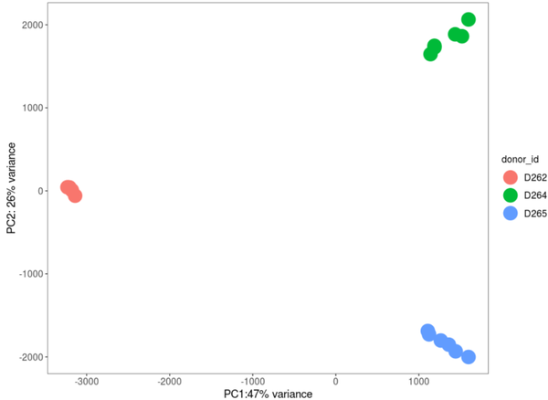
дЭМ
ЛљБОЗжВМЛЙЪЧВюВЛЖрЕФЃЌЃЌЃЌЃЌ
ПьШЅЪдвЛЪдбНЃЁ
ФуПЩФмЛЙЯыПД


https://blog.sciencenet.cn/blog-118204-1234759.html
ЩЯвЛЦЊЃКИДЯжnature communication PCAдЭМ|ДњТыЗжЮіЃЈвЛЃЉ
ЯТвЛЦЊЃКвЛИіRАќЭцзЊЕЅЯИАћУтвпзщПтЗжЮіЃЌЛЙФмгыSeuratЮоЗьЖдНг